39 conditional formatting data labels excel
Format Data Labels in Excel- Instructions - TeachUcomp, Inc. One way to do this is to click the "Format" tab within the "Chart Tools" contextual tab in the Ribbon. Then select the data labels to format from the "Current Selection" button group. Then click the "Format Selection" button that appears below the drop-down menu in the same area. How-to Make Conditional Data Labels for an Excel Dashboard Checkout the Step-by-Step Tutorial here: on How to conditionally hide and unhide data labels ...
VBA Conditional Formatting of Charts by Value and Label The category labels (XValues) and values (Values) are put into arrays, also for ease of processing. The code then looks at each point's value and label, to determine which cell has the desired formatting. The rows and columns are looped starting at 2, since the first of each contains an irrelevant label. The looping stops one count before the end.

Conditional formatting data labels excel
Changing the Color of a Data Label using IF Statement 1) Click on the data labels to highlight all the data labels, 2) Right-Click and select Format Data Labels, 3) Click on Number, 4) Go to the Format Code field *adapt the following to your needs* 5) [green] [>29]#.00; [<30] [Color 53]#.00 Click to expand... Hi Jawnne, I hope you're still lurking about on here. How to Create Excel Charts (Column or Bar) with Conditional Formatting ... Conditional formatting is the practice of assigning custom formatting to Excel cells—color, font, etc.—based on the specified criteria (conditions). The feature helps in analyzing data, finding statistically significant values, and identifying patterns within a given dataset. Conditional Formatting in Excel - Endsight First, highlight the values that we want formatted. Go to the Home tab, under the Styles section, and click Conditional Formatting. Excel has a variety of pre-set templates with rules for highlighting particular cell ranges, adding bars based on values, color scales, and even icons. Feel free to explore these different template rules.
Conditional formatting data labels excel. Use conditional formatting to highlight information Conditional formatting can help make patterns and trends in your data more apparent. To use it, you create rules that determine the format of cells based on their values, such as the following monthly temperature data with cell colors tied to cell values. r/excel - Is it possible to conditionally format Data Labels on a ... On a dynamic line chart, where Y-axis is scaled from 0-10 and X-axis is dates, is it possible to conditionally format Data Labels such that the colour of the data labels changes based on the data values that are plotted. For example, when numbers 0-3 are plotted on the dynamic chart above their data label's font colour turns red, and if numbers ... How to do conditional formatting of a label in Excel VBA Function ConditionalFormatNumber (n As Double) As String If n > 1000000 Then ConditionalFormatNumber = Format (n / 1000000, "$#,##0.00,,""M""") ElseIf n > 1000 Then ConditionalFormatNumber = Format (n / 1000, "$#,##0.00, ""K""") Else ConditionalFormatNumber = Format (n, "$#,##0.0") End If End Function Share answered Aug 24, 2017 at 9:13 Excel tutorial: How to use data labels Generally, the easiest way to show data labels to use the chart elements menu. When you check the box, you'll see data labels appear in the chart. If you have more than one data series, you can select a series first, then turn on data labels for that series only. You can even select a single bar, and show just one data label.
Conditional Formatting Shapes - Step by step Tutorial Let's see step by step how to create it: First, select an already formatted cell. In the picture below, we have created a little example of this. We will pay attention to the range D5:D6. You can see the rules in the Rules Manager window. We didn't make it overly complicated. How to create a chart with conditional formatting in Excel? - ExtendOffice Add three columns right to the source data as below screenshot shown: (1) Name the first column as >90, type the formula =IF (B2>90,B2,0) in the first blank cell of this column, and then drag the AutoFill Handle to the whole column; Excel bar chart with conditional formatting based on MoM change Click on any bar and press Ctrl+1 to make the Format Data Series task pane appear if it is not already showing. In the Series Options section, set the Gap Width to 50% to give the bars more presence and set the Series Overlap to 100%. Use the chart skittle (the "+" sign to the right of the chart) to remove the legend and gridlines. Custom Chart Data Labels In Excel With Formulas - How To Excel At Excel Follow the steps below to create the custom data labels. Select the chart label you want to change. In the formula-bar hit = (equals), select the cell reference containing your chart label's data. In this case, the first label is in cell E2. Finally, repeat for all your chart laebls.
Conditional format of chart labels - Excel Help Forum Whilst Conditional Formatting will not be pickup by the data labels there may be alternative approaches before reverting to VBA. Custom number format could control colour. Additional series in the chart could provide differently formatted labels. Can you post example and detail of what the CF is. Cheers Andy Register To Reply Conditional Formatting with Data Validation - Microsoft Tech Community Select the range in column C that you want to format, for example C2:C100. The first cell in the range (C2 in this example) should be the active cell in the selection. On the Home tab of the ribbon, select Conditional Formatting > New Rule... Select 'Use a formula to determine which cells to format'. Enter the formula Conditional formatting with formulas (10 examples) | Exceljet You can create a formula-based conditional formatting rule in four easy steps: 1. Select the cells you want to format. 2. Create a conditional formatting rule, and select the Formula option 3. Enter a formula that returns TRUE or FALSE. 4. Set formatting options and save the rule. How to add conditional colouring to Scatterplots in Excel Take the Y column and break it down into 3 columns A, B and C depending on the group the data point belongs to. To do this, we use the excel IF condition: IF (Condition, Value if True, Value if False) The condition we use is "label of the column = the group name".For example, for the first data point, in column A, we check if A = C.

How to Use Excel Custom Number Formatting – MBA Excel
Change the format of data labels in a chart To get there, after adding your data labels, select the data label to format, and then click Chart Elements > Data Labels > More Options. To go to the appropriate area, click one of the four icons ( Fill & Line, Effects, Size & Properties ( Layout & Properties in Outlook or Word), or Label Options) shown here.
The 'Art' of Formatting - Excel Conditional Formatting | Experts Exchange
Creating Conditional Data Labels in Excel Charts - YouTube We can make labels appear on our charts that don't have to do with the raw numbers that built the chart - and we can make them show up or not based on whatever conditions we want. In this tutorial,...

Automatically Remove Duplicate Rows in Excel
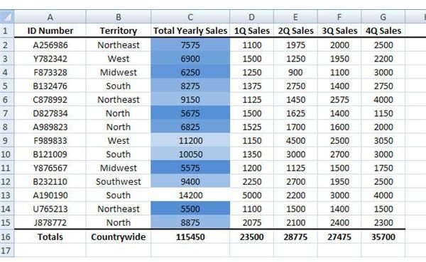
Excel conditional formatting Icon Sets, Data Bars and Color Scales Apply the conditional formatting icon set rule to Column A by clicking More Rules…, as explained above. Click the Reverse Icon Order button to change the order of icons. Select the Icon Set Only checkbox. For the cross icon, set >=5 (where 5 is the number of columns in your table, excluding the first "Icon" column).

Excel Course: Inserting Graphs
Conditional Formatting in Excel - a Beginner's Guide - GoSkills.com Click Conditional Formatting, then select Icon Set to choose from various shapes to help label your data. For this example, let's use the arrow icon set to show whether our highlighted data, the Variance column, has increased or decreased. Now, you'll see that the data has arrow icons accompanying their values in the cells.

HIGHLIGHT DUPLICATE VALUE IN EXCEL - Data analysis
How to change chart axis labels' font color and size in Excel? Sometimes, you may want to change labels' font color by positive/negative/ in an axis in chart. You can get it done with conditional formatting easily as follows: 1. Right click the axis you will change labels by positive/negative/0, and select the Format Axis from right-clicking menu. 2.

How to use Conditional Formatting in an Excel Sheet.
How to Use Conditional Formatting Based on Date in Microsoft Excel Open the sheet, select the cells you want to format, and head to the Home tab. In the Styles section of the ribbon, click the drop-down arrow for Conditional Formatting. Move your cursor to Highlight Cell Rules and choose "A Date Occurring" in the pop-out menu. A small window appears for you to set up your rule.

How to Create Multi-Category Chart in Excel - Excel Board
Custom Data Labels with Colors and Symbols in Excel Charts - [How To ... To apply custom format on data labels inside charts via custom number formatting, the data labels must be based on values. You have several options like series name, value from cells, category name. But it has to be values otherwise colors won't appear. Symbols issue is quite beyond me.

Create charts with conditional formatting – User Friendly
excel conditional formatting with data - Stack Overflow Select the cells/column(s) you want the conditional format applied to (for this example I assume you use column B:B) Check which cell is active - the "white" cell in the blue selection. (I assume it's B1) Create a new conditional format Home -> Conditional formatting -> New Rule; Select "Use a formula to determine which cells to format"

Conditional formatting in Excel 2010 | joy of data
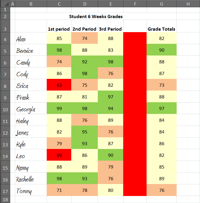
Excel Data Analysis - Conditional Formatting - tutorialspoint.com Follow the steps to conditionally format cells − Select the range to be conditionally formatted. Click Conditional Formatting in the Styles group under Home tab. Click Highlight Cells Rules from the drop-down menu. Click Greater Than and specify >750. Choose green color. Click Less Than and specify < 500. Choose red color.

33 Pivot Table Blank Row Label - Labels Database 2020
Conditional Formatting to Distinguish Between Labels and Numbers I want to conditionally format each cell, so that the text is yellow, the numbers are blue, and the blank cells are green. I tried by setting up a new rule under conditional formatting, then selecting "use a formula to determine which cells to format", then using some combinations of the if, istext, isnumber, etc. combinations. Please advise.
How to remove (temporarily hide) conditional formatting when printing in Excel?
Conditional Formatting in Excel - Endsight First, highlight the values that we want formatted. Go to the Home tab, under the Styles section, and click Conditional Formatting. Excel has a variety of pre-set templates with rules for highlighting particular cell ranges, adding bars based on values, color scales, and even icons. Feel free to explore these different template rules.

Avoid Duplicate Entries Using Data Validation In Excel – Excel-Bytes
How to Create Excel Charts (Column or Bar) with Conditional Formatting ... Conditional formatting is the practice of assigning custom formatting to Excel cells—color, font, etc.—based on the specified criteria (conditions). The feature helps in analyzing data, finding statistically significant values, and identifying patterns within a given dataset.

How to add New Rule Conditional formatting with custom formats in MS Excel #excelbasics #excel ...
Changing the Color of a Data Label using IF Statement 1) Click on the data labels to highlight all the data labels, 2) Right-Click and select Format Data Labels, 3) Click on Number, 4) Go to the Format Code field *adapt the following to your needs* 5) [green] [>29]#.00; [<30] [Color 53]#.00 Click to expand... Hi Jawnne, I hope you're still lurking about on here.
How to Create a New Conditional Formatting Rule in Microsoft Excel 2007 - Bright Hub
How to remove (temporarily hide) conditional formatting when printing in Excel?

How to Create Multi-Category Chart in Excel - Excel Board
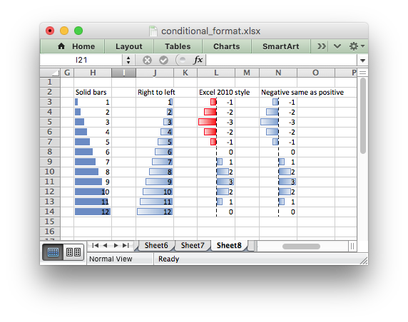
libxlsxwriter: Working with Conditional Formatting
Post a Comment for "39 conditional formatting data labels excel"