40 excel pie chart add labels
How to insert data labels to a Pie chart in Excel 2013 - YouTube This video will show you the simple steps to insert Data Labels in a pie chart in Microsoft® Excel 2013. Content in this video is provided on an "as is" basi... Edit titles or data labels in a chart - support.microsoft.com On a chart, click the label that you want to link to a corresponding worksheet cell. On the worksheet, click in the formula bar, and then type an equal sign (=). Select the worksheet cell that contains the data or text that you want to display in your chart. You can also type the reference to the worksheet cell in the formula bar.
Excel charts: add title, customize chart axis, legend and data labels ... Click the Chart Elements button, and select the Data Labels option. For example, this is how we can add labels to one of the data series in our Excel chart: For specific chart types, such as pie chart, you can also choose the labels location. For this, click the arrow next to Data Labels, and choose the option you want.

Excel pie chart add labels
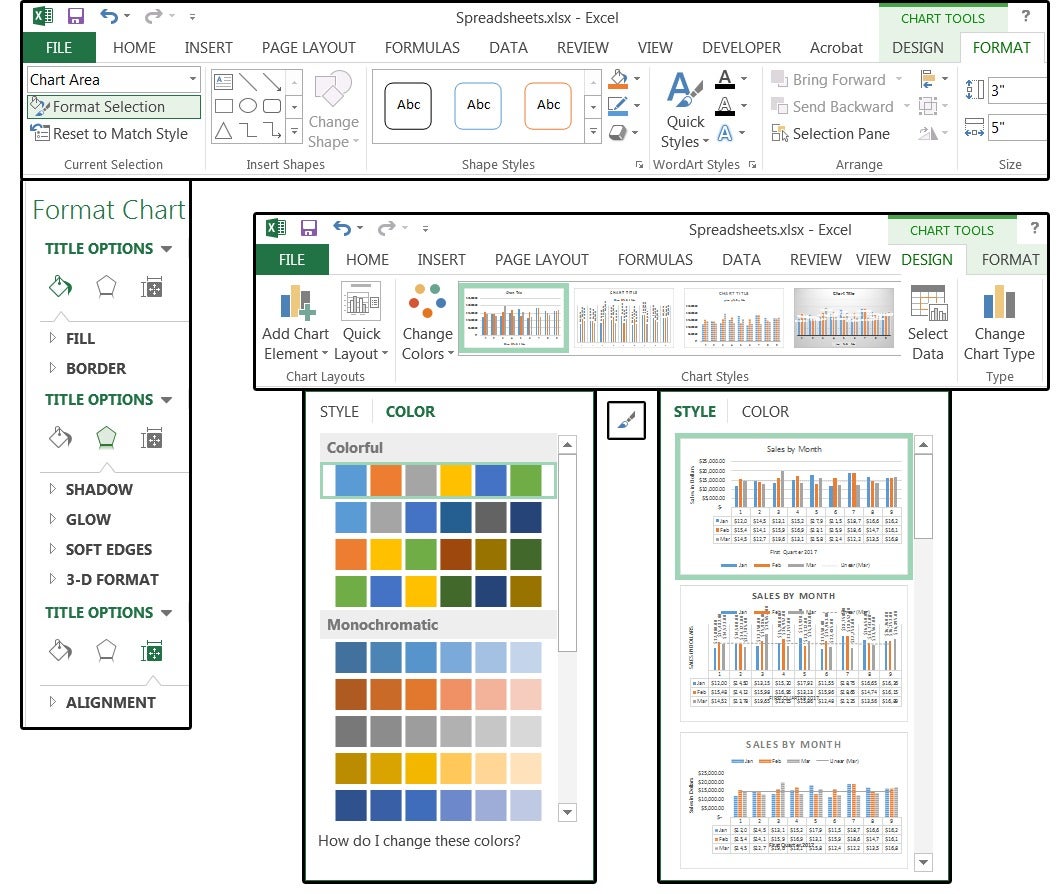
How to Show Percentage in Pie Chart in Excel? - GeeksforGeeks Jun 29, 2021 · Select a 2-D pie chart from the drop-down. A pie chart will be built. Select -> Insert -> Doughnut or Pie Chart -> 2-D Pie. Initially, the pie chart will not have any data labels in it. To add data labels, select the chart and then click on the “+” button in the top right corner of the pie chart and check the Data Labels button. How to Create and Format a Pie Chart in Excel - Lifewire Select the plot area of the pie chart. Right-click the chart. Select Add Data Labels . Select Add Data Labels. In this example, the sales for each cookie is added to the slices of the pie chart. Change Colors When a chart is created in Excel, or whenever an existing chart is selected, two additional tabs are added to the ribbon. Add / Move Data Labels in Charts - Excel & Google Sheets Adding Data Labels Click on the graph Select + Sign in the top right of the graph Check Data Labels Change Position of Data Labels Click on the arrow next to Data Labels to change the position of where the labels are in relation to the bar chart Final Graph with Data Labels
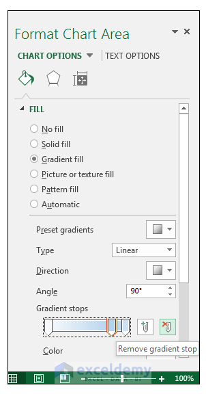
Excel pie chart add labels. How to display leader lines in pie chart in Excel? - ExtendOffice To display leader lines in pie chart, you just need to check an option then drag the labels out. 1. Click at the chart, and right click to select Format Data Labels from context menu. 2. In the popping Format Data Labels dialog/pane, check Show Leader Lines in the Label Options section. See screenshot: 3. excel - How can I add labels with percentage to a pie chart in Python ... import matplotlib.pyplot as plt import pandas as pd excel_file_path = "Chartdata.xlsx" df = pd.read_excel(excel_file_path) df_country = df.groupby(['Country']).sum() df_country ['Revenue'].plot.pie() plt.show() It reads an Excel file, checks if there are more locations for one country and if yes, sums the revenues for the locations in the same ... Pie Chart Examples | Types of Pie Charts in Excel ... - EDUCBA It is similar to Pie of the pie chart, but the only difference is that instead of a sub pie chart, a sub bar chart will be created. With this, we have completed all the 2D charts, and now we will create a 3D Pie chart. 4. 3D PIE Chart. A 3D pie chart is similar to PIE, but it has depth in addition to length and breadth. Add data labels and callouts to charts in Excel 365 - EasyTweaks.com Step #2: When you select the "Add Labels" option, all the different portions of the chart will automatically take on the corresponding values in the table that you used to generate the chart.The values in your chat labels are dynamic and will automatically change when the source value in the table changes. Step #3: Format the data labels.. Excel also gives you the option of formatting the ...
How to Create Bar of Pie Chart in Excel? Step-by-Step Excel lets us add our own customizations to the Bar of Pie chart. For example, it lets us specify how we want the portions to get split between the pie and the stacked bar. It also lets us specify whether we want to display data labels, what data labels we want to be displayed as well as what formatting and styling we want to apply to the labels. How to Make a Pie Chart in Excel & Add Rich Data Labels to The Chart! Creating and formatting the Pie Chart 1) Select the data. 2) Go to Insert> Charts> click on the drop-down arrow next to Pie Chart and under 2-D Pie, select the Pie Chart, shown below. 3) Chang the chart title to Breakdown of Errors Made During the Match, by clicking on it and typing the new title. Pie of Pie Chart in Excel - Inserting, Customizing, Formatting To add the data labels:- Select the chart and click on + icon at the top right corner of chart. Mark the check box containing data labels. Formatting Data Labels Consequently, this is going to insert default data labels on the chart. How to Make a Pie Chart in Excel (Only Guide You Need) To add labels to the slices of the pie chart do the following. 1 st select the pie chart and press on to the "+" shaped button which is actually the Chart Elements option Then put a tick mark on the Data Labels You will see that the data labels are inserted into the slices of your pie chart.
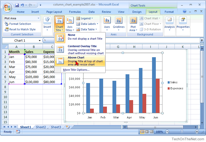
Adding 2nd Data Label Series to Bar of Pie Chart Re: Adding 2nd Data Label Series to Bar of Pie Chart. If you use 2 sets of the same data in the chart you can create 2 pie/bar charts, with one appearing on the secondary axis. Make sure the settings for bar/pie formatting are the same. Add data labels to each series. Format one to show names the other values. Add a pie chart - support.microsoft.com To switch to one of these pie charts, click the chart, and then on the Chart Tools Design tab, click Change Chart Type. When the Change Chart Type gallery opens, pick the one you want. See Also. Select data for a chart in Excel. Create a chart in Excel. Add a chart to your document in Word. Add a chart to your PowerPoint presentation How to Make a Pie Chart in Excel: 10 Steps (with Pictures) Apr 18, 2022 · Add your data to the chart. You'll place prospective pie chart sections' labels in the A column and those sections' values in the B column. For the budget example above, you might write "Car Expenses" in A2 and then put "$1000" in B2. The pie chart template will automatically determine percentages for you. Microsoft Excel Tutorials: Add Data Labels to a Pie Chart You should get the following menu: From the menu, select Add Data Labels. New data labels will then appear on your chart: The values are in percentages in Excel 2007, however. To change this, right click your chart again. From the menu, select Format Data Labels: When you click Format Data Labels , you should get a dialogue box.
How to Create and Label a Pie Chart in Excel 2013 : 8 Steps - Instructables
How to add axis label to chart in Excel? - ExtendOffice You can insert the horizontal axis label by clicking Primary Horizontal Axis Title under the Axis Title drop down, then click Title Below Axis, and a text box will appear at the bottom of the chart, then you can edit and input your title as following screenshots shown. 4.
Excel Charts: Excel Pie Chart With Individual Slice Radius
Excel custom pie chart labels - Microsoft Community Excel custom pie chart labels. I want to use a pivot table to make a pie chart out of this. I want each of the pieces of the pie to contain the number of entries and between parentheses the percentage. So in the "Yes" piece, there should be '3 (33%)'. Actually, if I hover the pie chart in Excel, I get exactly the notation O want!
Excel charts: Mastering pie charts, bar charts and more | PCWorld
How to add Axis Labels (X & Y) in Excel & Google Sheets Edit Chart Axis Labels. Click the Axis Title; Highlight the old axis labels; Type in your new axis name; Make sure the Axis Labels are clear, concise, and easy to understand. Dynamic Axis Titles. To make your Axis titles dynamic, enter a formula for your chart title. Click on the Axis Title you want to change
MS Excel 2007: How to Create a Column Chart
Add a DATA LABEL to ONE POINT on a chart in Excel All the data points will be highlighted. Click again on the single point that you want to add a data label to. Right-click and select ' Add data label '. This is the key step! Right-click again on the data point itself (not the label) and select ' Format data label '. You can now configure the label as required — select the content of ...
How to Make a Pie Chart in Excel & Add Rich Data Labels to The Chart!
Add or remove data labels in a chart - support.microsoft.com Click the data series or chart. To label one data point, after clicking the series, click that data point. In the upper right corner, next to the chart, click Add Chart Element > Data Labels. To change the location, click the arrow, and choose an option. If you want to show your data label inside a text bubble shape, click Data Callout.

How to Create Multi-Category Chart in Excel - Excel Board
Pie Chart in Excel - Inserting, Formatting, Filters, Data Labels To add Data Labels, Click on the + icon on the top right corner of the chart and mark the data label checkbox. You can also unmark the legends as we will add legend keys in the data labels. We can also format these data labels to show both percentage contribution and legend:- Right click on the Data Labels on the chart.
Post a Comment for "40 excel pie chart add labels"